Assisting Accountants with Similarity-based Machine Learning
Just last year, we released Boost to help accountants save time by automating their work. Boost instantly spots inconsistencies in their clients' ledgers, saving time and embarrassment! Every second, Digits sifts through every single transaction and performs a deep analysis. Boost alerts accountants if it finds errors like transactions in unexpected categories and suggests categories for transactions with missing categories.
The simplicity of the product is thanks to the powerful technology we built to make this possible.
With this three-part series, Digits' Machine Learning team provides a look behind the scenes at how it works.
In this first blog post, we will explain why machine learning is crucial for accounting and how we detect categories for banking transactions with similarity-based machine learning models. In parts two and three, we will dive into how we use machine learning to accelerate the interactions between accountants and their clients.
Why Machine Learning?
Machine learning is a versatile tool for many applications, including accounting. For example, if we want to categorize transactions correctly, we can look at similar transactions and mimic their existing categorizations. We could find highly-similar transactions through traditional statistical methods like determining the Levenshtein distance between the transaction descriptions, but those methods would have failed in the following scenarios:
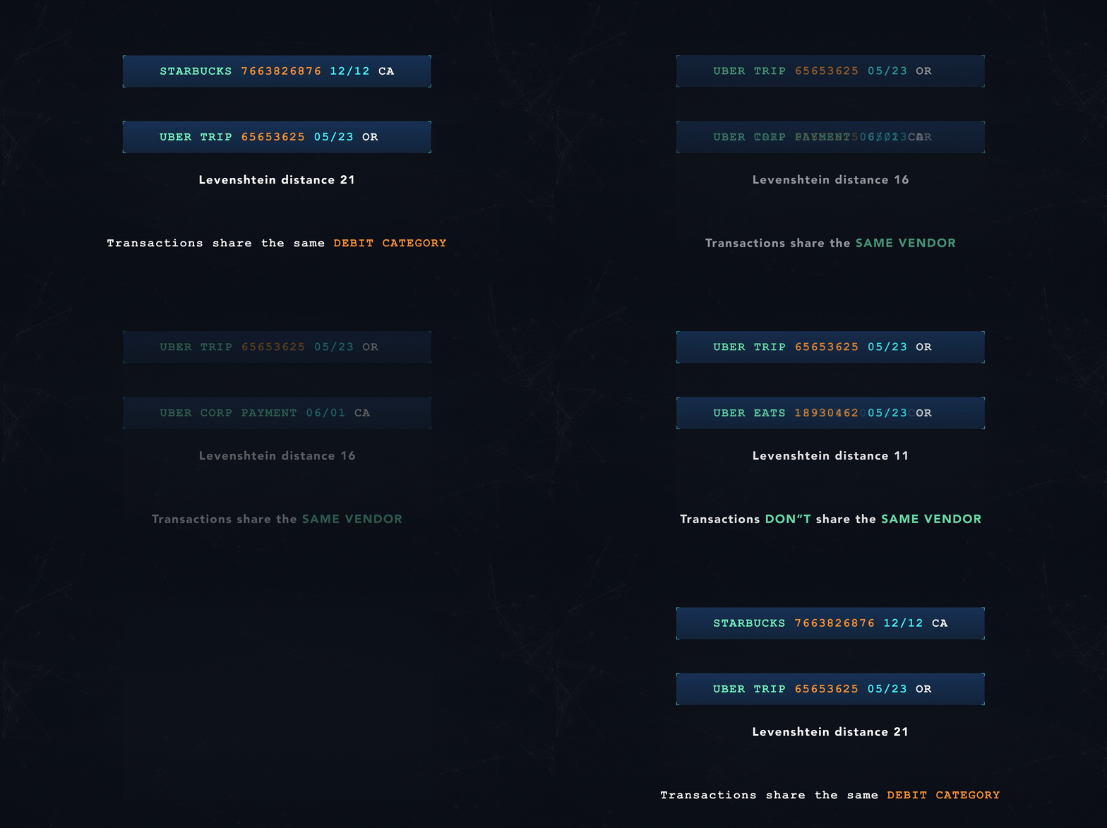
Because of the number of failure cases of traditional statistical methods, we decided to develop a custom machine learning-based solution.
Co-Piloting vs. Auto-Piloting
When people read about machine learning (ML) and artificial intelligence (AI), they often associate it with replacing the human who previously did the work. There are many scenarios where machine learning models can make decisions faster, at higher throughput, and with higher consistency (albeit with any bias inherent in the data) than humans. We can think of those scenarios as auto-pilot scenarios.
But the accounting world is so rich in human expertise that this belief is misguided. We should instead think about how we assist the experts, watching their backs by constantly checking for potential errors or making recommendations to speed up their custom workflows and interactions with their clients.
The accounting world is so rich in human expertise that we should instead think about how we assist the experts, not replace them.
Sanjeet Das, Product Manager at Digits
Rather than replacing human expertise, we see machine learning as the co-pilot to the accounting experts. What OpenAi's ChatGPT is for writers, Digits Boost is for accountants.
How are We Assisting Each Accountant?
Typically, a machine learning model can be trained to classify a transaction into a single accounting category. This is called classification-based machine learning. This prediction would always be the same if the input features were the same. However, two different accountants might want to classify the same transaction into two vastly different categories. For the transaction below, both options might be valid classifications:
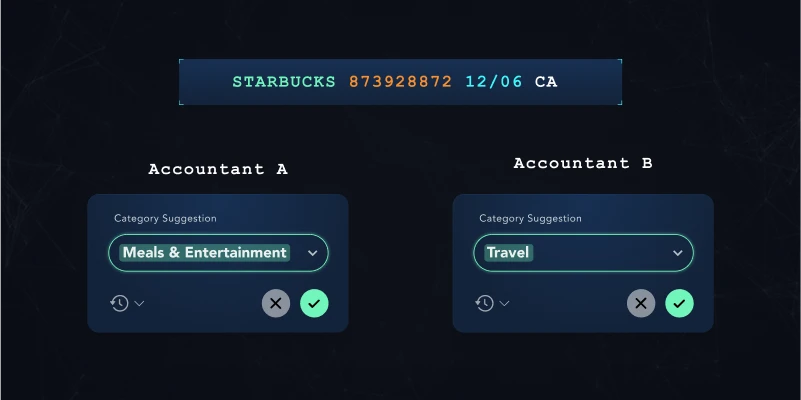
One accountant might classify it as Meals & Entertainment Expenses, while another might categorize it as a Travel expense because the expense happened while traveling.
How can machine learning assist in this scenario if the accountant's classifications are subjective and influenced by the client's context?
To assist accountants, we use a concept called similarity-based machine learning. Instead of classifying transactions into category buckets as we would have done with the classification-based machine learning approach, we teach a machine learning model to turn the banking transactions into mathematical vector embeddings, that capture the semantic relationships between transactions. The generated vector embeddings of related transactions are mathematically "close" to each other. That way, we can search a vector space of all transactions for related, historical transactions and derive information from past transactions about new, uncategorized transactions.
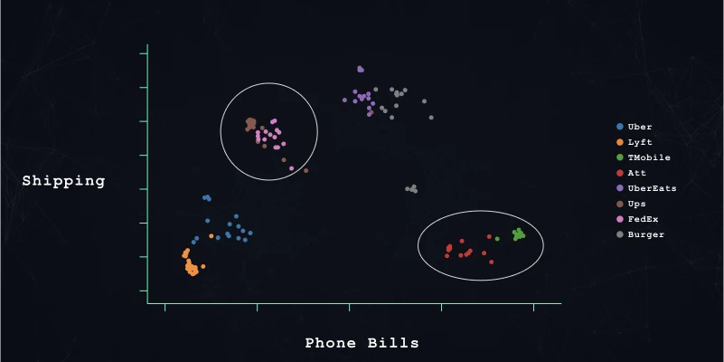
The figure below shows a 2-dimensional representation of our model-generated vector embeddings. Each dot represents a transaction originating from a particular vendor (each color represents a different vendor). The illustration shows that our embedding models learned to place similar transactions, for example, the Lyft and Uber transactions, close together. In addition, the machine learning model learned that Uber Eats is closer related to random Burger restaurants than its parent company Uber.
Our End-to-End Machine Learning System
From the moment a new transaction arrives at Digits to when we can recommend categories, every transaction goes through three stages:
Generate a vector embedding for the transaction
Search a vector space for related, historical transactions
Derive information from related, historical transactions

In the following sections, we will dive deeper into each of the three stages of our machine-learning system.
Generating Vector Embeddings for Transactions
We use similarity-based machine learning to generate content-aware embedding vectors. There are several machine learning techniques to create embedding vectors (e.g., auto-encoders), but we wanted to make sure that two transactions which seemingly have no features directly in common can be similar through their generated embedding vectors.
In each training pass in similarity-based machine learning, we train the model to encode three transactions. The model needs to encode each transaction such that: one transaction is close (positive sample), and one transaction is far apart (negative sample) from a third transaction (anchor sample).
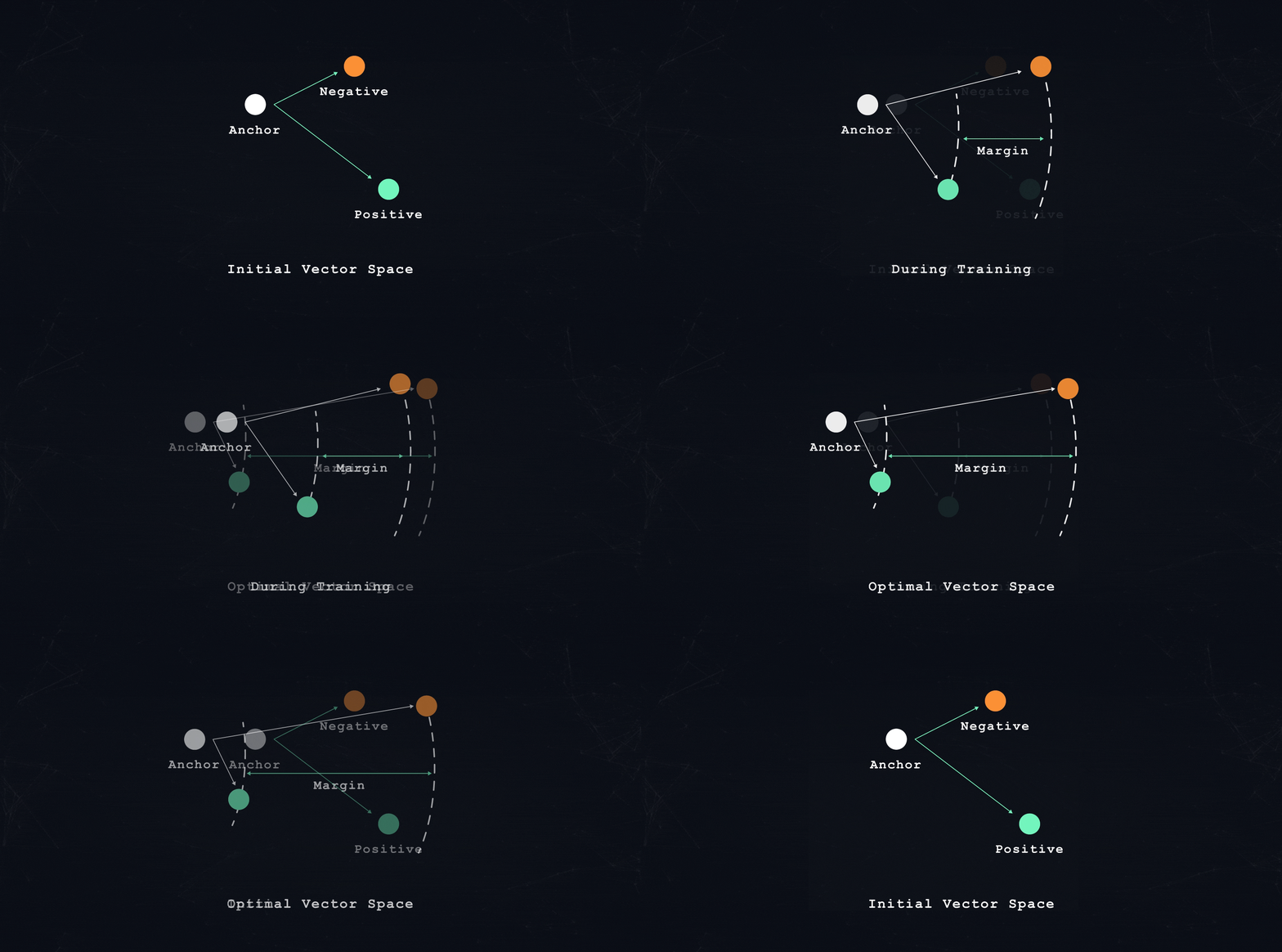
What is close and what is far apart depends on the overall training objective. A learning objective could be:
• Existing transaction categorizations where all transactions within the same category are considered positive samples and transactions from unrelated categories are considered negative samples.
• Associations between different vendors across transactions
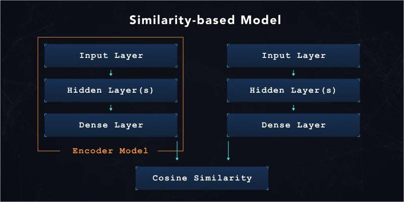
After the training of the similarity-based machine learning model, we only export the Encoder section of the trained model (shown below). We later deploy the Encoder model to our production machine learning endpoints to convert transactions into their representative embeddings.
While we implemented our own initial TensorFlow loss functions, we recommend the TensorFlow Similarity library, which provides various concept implementations and works well with our existing TensorFlow Extended (TFX) setup.
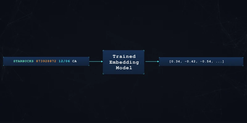
After training our embedding model for a specific objective, we can now generate embedding vectors with a fixed dimensionality for each transaction.
Search for Related Transactions
Mathematics provides several vector distance metrics to compare two vectors. The two most common distance metrics are:
Euclidean distances
Cosine distance
While Euclidean distance works well in smaller dimensional vector spaces, cosine distance is a good metric for comparing vectors of higher dimensions. However, cosine distance only compares two vectors based on their direction (angle) and not also on their vector magnitude. This is usually acceptable as the precise magnitude of the vectors becomes a much less relevant feature, while the angle between vectors is highly relevant as the space is relatively sparse. So cosine distance serves well here.
Another nice side effect of the cosine distance is that computationally it is the dot-product of two vectors once normalized.
Technically we can compute the distance between a given vector and all vectors through a brute-force approach. However, the brute-force approach will be computationally expensive once you reach a vector space containing millions of vectors.
To solve this scaling issue, approximate nearest neighbors (ANN) is a tool to reduce the time of comparing vectors. ANNs precompute an initial index or graph to accelerate the lookup during runtime. The pre-computation can speed up the lookup of similar vectors in production, but with the caveat of reduced accuracy.
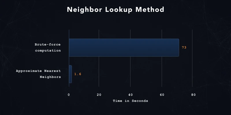
We can see the benefits of the approximations in the plots below. For computation comparison, we generated a vector index with 2 million embeddings and queried 128 test data points (shown below). The neighbor latency decreased by almost 98% when we switched from a brute-force look-up method to the nearest neighbor approximation (leafNodeEmbeddingCount 1000, leafNodesToSearchPercent 10%, distance metric: cosine, single item queries).
The recall of the approximated and the brute force results dropped slightly, but it is still very close (recall of the approximate results is 0.97 compared to the samples returned from the brute force queries).
Several algorithms exist to reduce this computation. In general, we can divide the most common algorithms into two camps:
Inverse indexes
Hierarchical Navigable Small World Graphs (HNSW)
The inverse index approach focuses on "bucketing" the embedding vectors into hash bins. The initial bucketing of the embedding vectors allows a faster look-up during runtime because similar vectors are retrieved based on the hash bin. A few algorithms exist for this approach, e.g., locality-sensitive hashing. The biggest downside of this approach is that once vectors are divided into hash bins, vectors can't be easily added, removed, or updated.
In recent years, HNSW has become more popular because it takes a different approach. Instead of creating an inverse index, HNSW builds a graph that can be efficiently searched. But even more importantly, it allows adding and updating vectors at runtime. We found that this is a tremendous benefit.
Several open-source libraries and managed services based on the HNSW algorithm exist to perform the ANN look-up in your application:
Google's ScaNN
Facebook's FAISS
Google Cloud's Vertex AI Matching Engine (based on ScaNN)
In case you are interested in a benchmark comparison between the different implementations, check out ann-benchmarks.com for detailed information.
We picked Google Cloud's Vertex Matching Engine as a managed service for our implementation. The matching engine supports automated sharding of extensive indexes and autoscaling when the service has to process a higher-than-standard throughput.
The following section provides an overview of how we integrate the managed service into our data pipelines.
Deriving Information from Related, Historical Transactions
Behind Digits, we run several data processing pipelines to give customers relevant suggestions at scale and in real-time. We have integrated the look-up of relevant, historical transactions in our batch and streaming pipelines.
For example, if a new transaction arrives at Digits, within seconds our streaming pipelines pick up the transactions, generate embedding vectors, look up related transactions, and process those transactions to extract the relevant information for the new transaction. If you want to learn more about our experiences with Google Cloud's Vertex Streaming Matching Engine, we highly recommend this introduction from Google in which we were able to share our experiences.
But the embedding vector queries also work at scale. Our batch pipelines process millions of transactions daily, and we heavily benefit from the auto-scaling capabilities of the Google Cloud's Vertex Matching Engine endpoints. In a future blog post, we will dive into how we consume the Vertex Matching Engine endpoint with Google Cloud Dataflow and how we optimize the services for optimal throughput.
Final Thoughts
At Digits, we assist thousands of accountants in their daily work through similarity-based machine learning and approximate nearest-neighbor searches. Both concepts combined let us elegantly handle the subjectivity of individual accountant decisions.
Our machine learning system consists of three stages: Generating the transaction embedding, looking up related transactions via cosine similarity distances, and then post-processing the associated transactions to extract the relevant information.
Approximate nearest neighbors algorithms perform well with vector spaces. In particular HSNW-based approximations provide additional production flexibility as vectors can be added, updated, and removed from the vector index during the runtime.
Further Reading
Check out these great resources for even more details on similarity-based machine learning and embedding vector databases:
Stay up to date with Digits
Unsubscribe anytime.


