Building Digits: Efficient Serving of Static Views with Google Cloud Spanner

At Digits, we strive to push the bounds of technology in order to deliver radically more useful, delightful software experiences for our customers. We’re excited to begin sharing a closer look at the technical foundations that underpin our products in a new series of blog posts called Building Digits. Without further ado…

Let’s talk about viewing complex data. One of our primary goals at Digits is to provide business owners with insightful and holistic views of their company’s finances, in substantially real-time.

Achieving this involves three major, independent steps:

We collect all of their relevant data from various sources, such as their QuickBooks, the financial institutions they bank with, their corporate credit card providers, etc.
We apply our algorithms and proprietary datasets to extend, interpret, and tease out meaning from all of their data.
We consolidate and aggregate the results into a holistic view that we then visualize for them on their dashboard.

Facts

We refer to the pieces of data that we receive from third party systems as Facts. This is not a judgement of the credibility or immutability of these systems, but rather a delineation of what is (and what is not) under our control.

For example, if we receive a transaction from an external source that looks like 05/12/20 - Taxi $15.05, we might classify it as Transportation. Later, we may receive another piece of information that leads us to believe that this transaction was actually a client expense, and is better classified as Meals & Entertainment. In this example, the transaction itself, the fact, did not change—but our interpretation of it did.

Computed Data

We refer to insights and analysis that are performed by Digits, based on all of the Facts that we have received, as Computed Data. In the example above, this involved a category classification of a transaction. In other cases, this might involve determining that two external pieces of information actually represent the same physical transaction, or detecting that a particular transaction tends to recur on a regular interval and that it should be treated as a subscription.

Benefits of Recomputation

One of the challenges with this model is that we receive new data from external systems constantly, and each new Fact we receive may shed more light on, or change our understanding of, earlier Facts we already recorded. The arrival of new Facts can impact virtually every aspect of our Computed Data. As a result, determining the subset of Computed Data that needs to be updated as a result of any new Fact arriving is non-trivially complex.

We’ve chosen to avoid this complexity by “recomputing the world.” We reconsider our entire set of Computed Data every time the set of Facts that it is based on changes in any way. This guarantees that Digits uses every piece of knowledge it has access to in order to model your business’s financial health at every moment, so it’s as accurate as it can possibly be.

Consistent Views of the World

The last core tenet of our architecture is our notion of a View. To us, a view of a customer’s data is the combination of all of the Facts for that customer at time T, as well as all of the Computed Data derived from that fact set. If the set of customer facts changes at time T+1, we’ll create a new view that represents that updated set of Facts and Computed Data.

When a customer loads our dashboard, we retrieve the latest available version of their view, and their experience is based on that view version for the remainder of the customer session.

What is the motivation for keeping their experience tied to a single, static view version? There are several:

Consistency. Assume that the arrival of a new fact causes us to re-label a subset of transactions as Meals & Entertainment instead of Transportation. It would be confusing to our customers if one or two of the transactions in this subset changed labels while others did not as they browsed the site, and even more confusing if additional transactions became recategorized incrementally as they loaded new pages.
Atomicity. Assume that we receive an external update that replaces one Fact with another. For example, a correction of a pending transaction with the actual, confirmed transaction and the date it posted. If a customer was looking at a page of transactions that included the pending transaction, and then clicked Next and loaded a new page that now, all of a sudden, included the confirmed version of the transaction, they would be confused why the transaction seemed to appear twice.

View Serving Architecture

For these reasons, we decided that our architecture would entail a system that is capable of loading a holistic view V1, serving a customer dashboard based on it, and then, at a later point in time, loading a new holistic view V2 and atomically switching to serving the next customer experience based on it. At yet another later point, after a configurable number of hours has elapsed, we want to unload view V1 as it is no longer needed to serve any customer experiences.

Frequency of Recomputation

For a given customer, we recompute their view whenever we detect that any of their Facts or Computed Data have changed. In practice, this varies from customer to customer but can roughly be assumed to be between 1 and 24 times per day.

Why Google Cloud Spanner?

After a detailed analysis of the major cloud platforms in 2018, we made the decision to begin building Digits on Google Cloud, and we have been quite pleased with that decision.

With the rest of our infrastructure within the Google ecosystem, it was natural to evaluate Spanner as a potential database technology, and there are quite a few aspects of Spanner that are beneficial to our use case:

Spanner is fully-managed and requires effectively zero overhead for database operations.
Its ability to automatically shard data via table interleaving was an appealing feature for us, as it allows us to prepare for high scale and still get the benefits of relational database features: efficient joins, foreign keys, etc.
Its ability to perform ACID transactions, as needed, was appealing to us from a financial data perspective.

Read-time SQL

There is a huge trade-off between pre-computing everything to reduce read latency (i.e. dashboard load time) while limiting development speed, versus biasing towards read-time computation, which permits rapid feature iteration on the frontend.

At Digits’ current stage, we want to be in the middle of this spectrum — have low read latencies for a great user experience, but still be able to quickly iterate and perfect new features based on customer feedback. In order to support this model, whichever solution we chose for serving our views would have to support read-time SQL.

Sharding and Interleaving

Once it became clear that read-time SQL support was a requirement, we also wanted to be sure that the database solution we selected would easily scale with us as we grew. Traditional RDBMS systems have trouble scaling join performance once the data set can no longer fit on a single node, and many NoSQL key-value stores address the scalability concern by sacrificing join support entirely.

Spanner’s interleaving/sharding design is a nice balance between these two ends of the spectrum. While all data for a given set of parent-child tables does not need to fit on a single node, rows that share the same root key are guaranteed to be co-located on a node. This allows for fast joins within a parent-child hierarchy and aside from defining the interleaving model in the schema, it happens without the developer’s involvement.

Alternative Solutions

Combined, these constraints of easy scalability, low latency reads, and support for relational SQL eliminate quite a few otherwise appealing solutions. For example:

Cassandra and Redis are both great for serving precomputed views, but do not support read time aggregations via SQL. (Cassandra does support a SQL API but not read-time aggregation via SQL)
MySQL and Postgres are great for relational querying and read-time aggregation, but are challenging to scale, as sharding data across clusters is left to the engineer/operator.
Google BigQuery is great for all kinds of SQL analytics querying but is not designed to serve low latency, customer-facing dashboard reads.

Based on all of these factors, we elected to implement our view architecture on Spanner.

Implementing Views in Spanner

As we developed our view implementation, one of the challenges that we had to overcome was Spanner’s 20,000 cell mutation limit. The limit caps the number of cells (rows * columns-per-row) that can be inserted/updated in a single transaction.

This limit presented challenges on both the view loading side and the view unloading (deleting) side.

View Loading

On the view loading side it meant that as we computed views for a given customer, we could not guarantee that we could load the entire view into the database atomically. Additionally, it is non-trivial for the implementer to know whether a particular transaction would hit this limit or not as they would need to keep track of all of the cells impacted by the generated mutations or the DML statement.

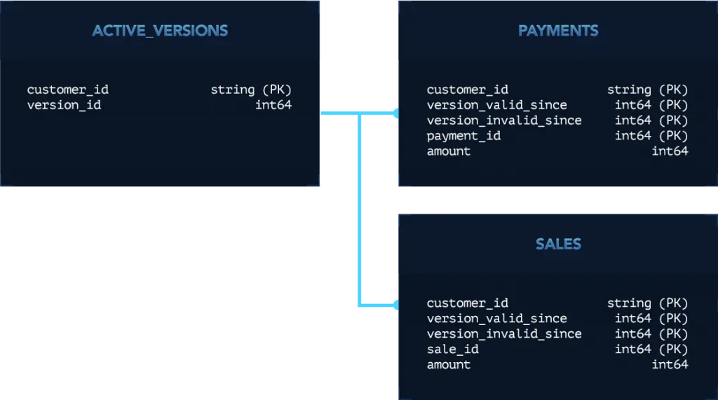
To address this, we created a view version table that is independent of the tables that actually store the view data. This table is a simple mapping from a customer id to a version identifier. This version column is also set on all rows of the actual view data tables.

For example, a small subset of our view schema may look like this:

The queries that power our dashboard can either serve a view for a particular, known, version or consult the active versions table to see which version is the latest (our version_ids increase monotonically).

Our view loading process, for a given customer, then looks like this:

Load all parts of the view in independent transactions of roughly 100 rows each (conservative to stay well-clear of the mutation limit).
Once all parts of the view have been successfully loaded, update the view version table to denote the newest active version.

This process ensures that a new view will be served atomically in its entirety, because no query will be aware of its existence until the view version table has been updated. At the same time, existing customer sessions can continue to experience our dashboard against the view version which was active at the start of their session.

View Unloading

The same 20,000 cell mutation limit applies to data deletion. Spanner does support a Partitioned DML alternative that was appealing for this use case, however we found two limitations with it:

Every time we load a new view, it effectively invalidates a similarly sized older view, and this amounts to tens of thousands of rows in need of deletion. This has a significant impact on CPU load. Spanner tombstones rows that are marked as deleted, which makes them invisible to all queries, and then reclaims the disk space in an asynchronous process. However, in our experience both the tombstoning and the reclamation process place a non-trivial load on the CPU and can thus impact read latency of customer facing queries.
The partitioned DML alternative that is documented to not be constrained by the 20,000 cell mutation limit still fails intermittently with the 20,000 cell mutation limit error.

Efficient Incremental Views

To address the deletion constraint, we analyzed the insertions and deletions that we were performing as part of view loading/unloading and confirmed what we expected: the vast majority of rows stay the same from one view version to the next. All we had to do was invest in being able to easily identify the rows that actually changed, and only inserting and removing the deltas.

(It is important to note that while determining which pieces of our Computed Data for a given customer need to be updated because we received new Facts is non-trivially complex, comparing two fully computed views to each other and determining which rows have been updated, removed, or created is quite straightforward.)

The output of this comparison can then be used as follows:

Each row in the current active version is determined to:

Still be relevant
Be removed for all view versions going forward

Each row in the newly computed version is determined to:

Already be present in the active view version
Be added for all view versions going forward

For most normal operations, 99% of rows in both the existing version and the new version are determined to be identical, and thus no-ops.

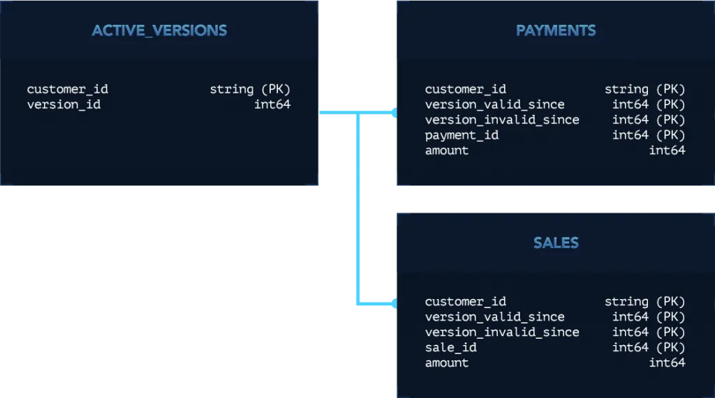
To support this, we modified our view tables to have two version-related columns, version_valid_since and version_invalid_since, and updated all queries with two WHERE conditions. For example, continuing with the example schema above, our modified schema would look like this:

Finally, we implemented version diffing in a generic way, such that it can be applied to all of our view tables without additional work.

With this in place, we now have to insert and delete 99% less data from Spanner than we did when we were fully loading/unloading every view.

Schema Design for Scale

One unintuitive aspect of Spanner’s secondary indexes (indexes you explicitly add to tables as opposed to the index you implicitly get for the primary key), is that if a query which hits the index selects a column that is neither a part of the index nor explicitly stored on the index, Spanner must perform an implicit join from the secondary index back to the base table. This makes sense once you accept the fact that the index is stored as an independent structure from the table that it is indexing.

Unfortunately, this join may be non-trivial in cost, particularly when a lot of data is being selected.

To avoid secondary-index-to-base-table join costs, we have explored two options:

Carefully designing our tables’ primary keys in such a way that most common queries only require the implicit primary key index.
Creating secondary indexes that are less generic and more tailored to specific query patterns by including all of the columns selected by that query in their STORING clauses.

The second option has a higher maintenance cost as it potentially requires updating indexes when new columns are added to tables (if these new columns are selected by queries which indexes are tailored for) or when query patterns are added for product reasons. As a result, we prefer the first approach whenever possible.

For example, if the majority of queries against a table will involve restricting the result set by time, then we consider adding the column that represents time to be part of the primary key, even if it logically is not required to be in the primary key.

Sharding

Spanner’s interleaving support allows for schema design that makes your database straightforward to scale while still supporting efficient joins on data that is commonly joined together. These two properties are often very difficult to achieve in tandem with relational databases.

Interleaving lets you to signal to Spanner that all hierarchical data spanning multiple tables, rooted at a particular root row, should be colocated together. Building on our schema examples above, it might be appealing to interleave all of our view data under the customers table. This would mean that all view data for a given customer would be colocated—a property that makes sense since we often want to show a customer various parts of their data, while we never want to join data from multiple customers together.

The schema for the customers table as well as the view tables above may then look like this:

CREATE TABLE customers (
    customer_id STRING(MAX) NOT NULL,
    name STRING(MAX)
) PRIMARY KEY (customer_id);

CREATE TABLE active_versions (
    customer_id STRING(MAX) NOT NULL,
    version INT64 NOT NULL
) PRIMARY KEY (customer_id), INTERLEAVE IN PARENT customers ON DELETE CASCADE;

CREATE TABLE payments (
    customer_id STRING(MAX) NOT NULL,
    version_valid_since INT64 NOT NULL,
    version_invalid_since INT64,
    payment_id INT64 NOT NULL,
    amount INT64 NOT NULL,
) PRIMARY KEY (customer_id, version_valid_since, payment_id), INTERLEAVE IN PARENT customers ON DELETE CASCADE;

CREATE TABLE sales (
    customer_id STRING(MAX) NOT NULL,
    version_valid_since INT64 NOT NULL,
    version_invalid_since INT64,
    sale_id INT64 NOT NULL,
    amount INT64 NOT NULL,
) PRIMARY KEY (customer_id, version_valid_since, sale_id), INTERLEAVE IN PARENT customers ON DELETE CASCADE;

This schema might work well, but there is another factor to keep in mind: the size of all data that is interleaved under a single root has a hard limit in Spanner of 4 GB. To avoid approaching this limit, we might further restrict the data that is co-located.

For example, if we know that there are pieces of data that will never be joined with each other, then there is no reason for them to be co-located on the same node. Building on our scenario above, imagine that payments and sales are shown in totally separate parts of our dashboard and would never need to be joined together. If that were the case, then interleaving and thus colocating the view data for both of these tables, for a given customer, under the same customer_id row would make that row unnecessarily large.

To address this, we could add a table in between customers and payments/sales that would facilitate better sharding. The new table might look like:

CREATE TABLE customer_view_types (
    customer_id STRING(MAX) NOT NULL,
    view_type STRING(MAX)
) PRIMARY KEY (customer_id, view_type) INTERLEAVE IN PARENT customers ON DELETE CASCADE;

And the payments and sales tables would be updated to look like:

CREATE TABLE payments (
    customer_id STRING(MAX) NOT NULL,
    view_type STRING(MAX),
    version_valid_since INT64 NOT NULL,
    version_invalid_since INT64,
    payment_id INT64 NOT NULL,
    amount INT64 NOT NULL,
) PRIMARY KEY (customer_id, view_type, version_valid_since, payment_id), INTERLEAVE IN PARENT customer_view_types ON DELETE CASCADE;

CREATE TABLE sales (
    customer_id STRING(MAX) NOT NULL,
    view_type STRING(MAX),
    version_valid_since INT64 NOT NULL,
    version_invalid_since INT64,
    sale_id INT64 NOT NULL,
    amount INT64 NOT NULL,
) PRIMARY KEY (customer_id, view_type, version_valid_since, sale_id), INTERLEAVE IN PARENT customer_view_types ON DELETE CASCADE;

In Production

While there were a few limitations to work around, and special care must be taken in both schema design and query design to maintain high performance, Spanner has performed well in production as our customer base has scaled to billions of dollars in transaction value.

Incremental static views provide an optimal balance between dashboard consistency, read-time latency, continual re-computation based on new data, and developer productivity, and Spanner’s ease of scalability via auto-sharding and interleaving has made this architecture very low-overhead to operate.

Join the Team

Static view serving at scale is just one of countless technical challenges we’ve faced while building Digits, and we’re pushing the boundaries at every layer of the stack.

If you’re interested in crafting the next generation of financial software, we’re hiring, and we’d love to meet you! See our open positions here.